PC-SAFT
PC-SAFT
The Perturbed-Chain Statistical Associating Fluid Theory (PC-SAFT) equation of state is available as PCSAFT. It is constructed with init_pcsaft.
Use it when a molecular-size/chain description and suitable PC-SAFT parameter sets are available, for example for non-associating chain molecules. Rather than treating a molecule as one object with a single covolume, PC-SAFT represents it as connected segments. Crowding resists compression, connectivity changes the reference fluid, and dispersion attractions lower the free energy.
The name includes “associating”, but this implementation has no association term. It is not a general-purpose water/alcohol model, nor does it add a separate polar contribution. A parameter set fitted for another PC-SAFT variant may rely on terms absent here.
The following is a constructor snippet, with parameter arrays defined below:
use yaeos, only: pr, PcSaft, init_pcsaft

type(PcSaft) :: model

model = init_pcsaft(m, sigma, epsilon_k, kij)
Theory
PC-SAFT is a residual Helmholtz model based on a perturbation expansion around a
hard-chain reference fluid. Let be total residual Helmholtz energy,
the number of molecules, Boltzmann’s constant, and absolute
temperature. Write , with the total
mole amount and the gas constant. Superscripts hc, hs, and disp
mean hard chain, hard sphere, and dispersion, respectively. Then
Hard-chain contribution
Let be molecular mole fraction, the dimensionless segment count, and its mixture average. Let be the dimensionless same-component hard-sphere contact value. The hard-chain term already combines the hard-sphere reference and connectivity:
Do not add a separate chain term again. Here is the dimensionless hard-sphere reference per segment, not a second whole-molecule Helmholtz contribution. For the size mixture it uses the following mixture hard-sphere expression (reducing to Carnahan-Starling for equal diameters). The moments are defined immediately below:
Let be molecular number density in Å⁻³, the segment
diameter in Å, and the segment energy parameter in K
(the input epsilon_k). Define the temperature-dependent effective diameter
. The moments are
In particular, , not . The packing fraction is dimensionless; the other moments have units Å to the power . The contact function uses effective diameter , not the uncorrected :
Chain contribution
The chain contribution is included in the hard-chain term through the factors. It accounts for the connectivity of the segments that form each molecule.
Dispersion contribution
The unlike diameter is in Å, the unlike energy parameter is in K, and is a dimensionless binary correction. The combining rules are
The dimensionless integrals and and reference compressibility correction depend on packing fraction and mean chain length. The implemented second-order dispersion expression is
The temperature factors and must not be omitted. Define the
dimensionless polynomial coefficients , from
the Gross-Sadowski tables (stored in the source as a_coeffs and b_coeffs,
each with three rows). Then
with the mean-segment dependence
and the same form for . The packing fraction is the third moment , and
Although the polynomial coefficients have no explicit temperature argument, the integrals are not temperature-independent at fixed density: uses the temperature-dependent . Dispersion uses , while the packing and contact terms use ; these are different quantities in this implementation.
Units
The internal number density is in molecules per ų, and the parameters are (segments per molecule), (segment diameter in Angstrom), and (segment energy in K). The binary interaction matrix is dimensionless.
The model parameters are:
| Argument | Meaning | Units |
|---|---|---|
m |
Number of segments per molecule | - |
sigma |
Segment diameter | Angstrom |
epsilon_k |
Segment energy divided by Boltzmann’s constant | K |
kij |
Optional binary interaction matrix | - |
m, sigma, and epsilon_k are arrays with one entry per component. kij
is an optional nc x nc matrix; when it is omitted, all binary interaction
parameters are set to zero.
Use positive m, sigma, and epsilon_k, with consistent parameter provenance.
m is an effective segment count and may be noninteger. All arrays and both
axes of kij must use the same component order. Supply symmetric binary
corrections with zero diagonals; do not transfer cubic-EOS kij values to
PC-SAFT without validation.
The public property API still uses mol, total L, K, and bar, not ų:
the code converts number density using Avogadro’s constant and
1 L = 10^27 Å^3. sigma is the exception to the usual macroscopic unit set;
it is not in metres or litres.
Example
The following complete program uses the methane/n-butane parameter set shown
in Gross and Sadowski (2001). The zero-binary-correction mixture is a starting
point, not a fitted prediction for this mixture. It first evaluates pressure
at a prescribed homogeneous state and then asks a separate solver for a bubble
point at the same temperature. At a bubble point n/sum(n) is the liquid
composition and sat%y is the incipient vapor composition.
program pcsaft_example
   use yaeos, only: pr, PcSaft, init_pcsaft
   use yaeos, only: EquilibriumState, saturation_pressure
   use, intrinsic :: ieee_arithmetic, only: ieee_is_finite
   implicit none

   type(PcSaft) :: model
   type(EquilibriumState) :: sat
   real(pr) :: m(2)
   real(pr) :: sigma(2)
   real(pr) :: epsilon_k(2)
   real(pr) :: n(2)
   real(pr) :: T
   real(pr) :: V
   real(pr) :: P

   ! Methane and n-butane
   m = [1.0000_pr, 2.3316_pr]
   sigma = [3.7039_pr, 3.7086_pr]
   epsilon_k = [150.03_pr, 222.88_pr]

   model = init_pcsaft(m, sigma, epsilon_k)

   n = [0.4_pr, 0.6_pr]
   T = 300.0_pr
   V = 10.0_pr ! total L for one mole

   call model%pressure(n, V, T, P)
   print *, "Pressure: ", P, " bar"

   sat = saturation_pressure(model, n, T, kind="bubble")
   if (.not. ieee_is_finite(sat%P)) error stop "Nonfinite bubble pressure"
   if (sat%P <= 0.0_pr) error stop "Invalid bubble pressure"
   if (.not. all(ieee_is_finite(sat%y))) error stop "Nonfinite vapor composition"
   print *, "Saturation pressure: ", sat%P, " bar"
   print *, "Vapor composition: ", sat%y
end program pcsaft_example
At this low-density pressure-evaluation state, compare pressure with the
ideal-gas value sum(n)*R*T/V (R is exported by yaeos). Increase volume
to check approach to the ideal-gas limit. Pressure evaluated at a chosen volume
is not the saturation pressure, and need not equal sat%P.
The finite/positive checks are necessary but insufficient: also check
normalization, nonnegative phase compositions, distinct liquid/vapor roots
away from criticality, and equality of component fugacities. See the
saturation guide.
How init_pcsaft works
PC-SAFT is a residual Helmholtz model, but many yaeos routines also need
critical constants and acentric factors. init_pcsaft computes them from the
PC-SAFT parameters:
find_critical_points_all_componentscalculates the pure-component critical temperature, pressure, and volume from the PC-SAFT equation.Psat_pureevaluates the saturation pressure at .- The acentric factor is obtained from the definition .
This initialization is more expensive than constructing a cubic model, because it requires solving the critical point and a saturation point for each component. It is done once per model.
These are model-predicted critical constants, not additional experimental
inputs. The initializer obtains a converged array internally but does not
return it to callers. Check that model%components%Tc, %Pc, and %w are
finite and physically plausible before trusting downstream initial guesses.
Unusual parameter sets may fail during this initialization, before any mixture
property call is made.
A second example: saturation-temperature scan
program pcsaft_saturation_scan
   use yaeos, only: pr, PcSaft, init_pcsaft
   use yaeos, only: EquilibriumState, saturation_temperature
   use, intrinsic :: ieee_arithmetic, only: ieee_is_finite
   implicit none

   type(PcSaft) :: model
   type(EquilibriumState) :: sat
   real(pr) :: m(2)
   real(pr) :: sigma(2)
   real(pr) :: epsilon_k(2)
   real(pr) :: n(2)
   real(pr) :: Pvals(5)
   integer :: i

   m = [1.0000_pr, 2.3316_pr]
   sigma = [3.7039_pr, 3.7086_pr]
   epsilon_k = [150.03_pr, 222.88_pr]

   model = init_pcsaft(m, sigma, epsilon_k)

   n = [0.4_pr, 0.6_pr]

   Pvals = [1.0_pr, 5.0_pr, 10.0_pr, 20.0_pr, 40.0_pr]

   do i = 1, size(Pvals)
      sat = saturation_temperature(model, n, P=Pvals(i), kind="bubble", t0=250.0_pr)
      if (.not. ieee_is_finite(sat%T)) error stop "Nonfinite saturation temperature"
      if (sat%T <= 0.0_pr) error stop "Invalid saturation temperature"
      print *, "P =", Pvals(i), "bar, Tsat =", sat%T, "K"
   end do
end program pcsaft_saturation_scan
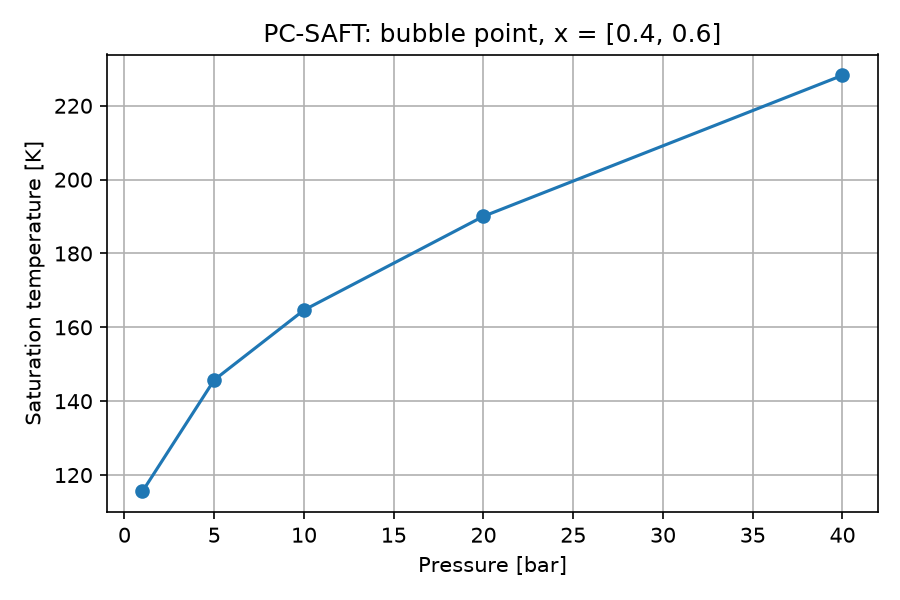
This retained illustration is a scan of bubble temperature, not a phase
envelope or a validation dataset. The program is complete and each point is a
separate nonlinear solve. A fixed t0 may fail in another pressure range;
continuing from the previous converged point can be more reliable.
Implementation details
PcSaft extends ArModelTapenade. The residual Helmholtz energy and its
derivatives are generated with Tapenade, so the model provides the full set of
first and second derivatives required by the phase-equilibrium routines.
The model implements:
ar,ar_d,ar_b,ar_d_b, andar_d_dfor the Tapenade interface.- A specialized
volumesolver based on Michelsen’s method. get_v0, which returns the total segment volume. This is the physical lower scale used to initialize the liquid root, not a universal stable-liquid bound.
The PC-SAFT contribution contains the hard-sphere, chain, and dispersion terms of the Gross-Sadowski formulation. The current implementation does not include the association term, so it should not be used for associating fluids such as water or alcohols without an additional model.
Notes and recommendations
- Use the model-specific units:
sigmain Angstrom andepsilon_kin kelvin. - Provide
kijfor mixtures when binary interaction parameters are available. Use the usual symmetric convention with zero diagonals. - The segment number
mcan be a real number; it is not restricted to integers. - The initialization calculates critical constants numerically. If a component
does not have a stable critical point under PC-SAFT,
init_pcsaftwill not produce reliable acentric factors. - For associating fluids, the association contribution is not implemented in this version.
- The model is significantly more expensive than a cubic equation of state. For phase-envelope calculations, provide good initial guesses to the saturation and flash routines.
Finite positive pressure does not establish phase stability. The packing fraction must stay below the hard-sphere singularity at one, and approaching that singularity is not a route to a trustworthy compressed-liquid prediction. Distinguish missing physical contributions or unsuitable parameters from volume-root and phase-equilibrium convergence failures.
Next reading
See the EOS property guide, thermodynamic fundamentals, saturation points, and flash calculations. For a lower-input baseline, compare the cubic models using the same state and composition.
References
- Gross, J., & Sadowski, G. (2001). Perturbed-Chain SAFT: An Equation of State Based on a Perturbation Theory for Chain Molecules. Industrial & Engineering Chemistry Research, 40(4), 1244-1260.