GERG2008
GERG2008
The GERG2008 equation of state is a multifluid model for natural-gas mixtures. It is based on the reduced Helmholtz energy and is the reference model of the GERG2008 monograph by Kunz and Wagner.
Use it when your mixture is built from the 21 components the model supports and you want a well-documented reference calculation without assembling critical constants, binary interaction parameters or a mixing rule yourself. Compared with a cubic EOS, the model is more expensive to evaluate and it comes with a fixed parameterization: you cannot supply your own pure-component or binary data.
This page explains what the model computes, what data it needs (very little), how to build it, and how to read its results.
Theory
Why a Helmholtz energy
An equation of state relates pressure, volume and temperature. A Helmholtz
energy model stores the same information in a thermodynamic potential whose
derivatives give the other properties. yaeos uses the residual Helmholtz
energy : the difference between the real fluid and an ideal gas at the
same amount, volume and temperature.
Let be the amount of component in mol, the total amount, the mole fraction, the absolute temperature in K, and the total volume in L. The residual Helmholtz energy is
where is the dimensionless reduced residual Helmholtz energy and is the gas constant in bar L/(mol K). The reduced density and reduced inverse temperature are
with the molar density in mol/L, the reducing density in mol/L, and the reducing temperature in K (not the reduced temperature used on the cubic pages). Each pure fluid keeps its own accurate Helmholtz equation, and the composition-dependent and combine them into a mixture: this is the “multifluid” idea.
The mixture residual energy
The implementation splits the reduced residual energy into a pure-fluid part and a binary departure part:
where is the number of components. The are the tabulated pure-component residual Helmholtz energies of component , and is the departure function of the pair . The dimensionless factor scales a pair’s departure function; it is zero for pairs that have no departure function, in which case the pair contributes nothing to this sum.
Composition-dependent reducing functions
The reducing volume (L/mol) and reducing temperature (K) are built from the pure-component critical data and the binary reducing parameters :
Here is the critical volume of component in L/mol, its critical temperature in K, and its critical density in mol/L. Every binary pair has reducing parameters, so the mixture critical behavior changes with composition even when no departure function is present.
Which pairs have a departure function
Only some pairs carry a binary departure function. In the tabulated data the following pairs have one (the numbers are the internal GERG2008 table indices, listed in the component table further down; the coefficients of each function are on the GERG2008 parameters page):
| Pair | Components | |
|---|---|---|
| 1-2 | methane + nitrogen | 1 |
| 1-3 | methane + carbon dioxide | 1 |
| 1-4 | methane + ethane | 1 |
| 1-5 | methane + propane | 1 |
| 1-6 | methane + n-butane | 1 |
| 1-7 | methane + isobutane | 0.771035405688 |
| 1-15 | methane + hydrogen | 1 |
| 2-3 | nitrogen + carbon dioxide | 1 |
| 2-4 | nitrogen + ethane | 1 |
| 4-5 | ethane + propane | 0.130424765150 |
| 4-6 | ethane + n-butane | 0.281570073085 |
| 4-7 | ethane + isobutane | 0.260632376098 |
| 5-6 | propane + n-butane | 0.0312572600489 |
| 5-7 | propane + isobutane | -0.0551609771024 |
| 6-7 | n-butane + isobutane | -0.0551240293009 |
For every other pair (for example methane + water, methane + n-pentane, carbon dioxide + water, or anything involving helium or argon) the mixture interaction is described only by the composition-dependent reducing functions. This is a property of the parameterization, not a numerical failure, and it is worth knowing before using the model for a mixture that relies on a strong unlike attraction, such as a water-bearing gas.
Data requirements
The only input the model needs is the list of components. Pure-component coefficients, binary departure functions, binary reducing parameters and the critical constants all come from the built-in GERG2008 tables, listed in full on the GERG2008 parameters page. The model type is Gerg2008 and it is built with gerg_2008.
The identifiers are fields of the public object G2008Components:
| Identifier | Component | Identifier | Component |
|---|---|---|---|
methane |
Methane | nonane |
n-Nonane |
nitrogen |
Nitrogen | decane |
n-Decane |
carbon_dioxide |
Carbon dioxide | hydrogen |
Hydrogen |
ethane |
Ethane | oxygen |
Oxygen |
propane |
Propane | carbon_monoxide |
Carbon monoxide |
nbutane |
n-Butane | water |
Water |
isobutane |
Isobutane | hydrogen_sulfide |
Hydrogen sulfide |
npentane |
n-Pentane | helium |
Helium |
isopentane |
Isopentane | argon |
Argon |
nhexane |
n-Hexane | ||
nheptane |
n-Heptane | ||
noctane |
n-Octane |
Note
The component names are fields of G2008Components, not integer constants.
Use G2008Components%methane, for example, not methane.
The order of the identifiers is the order of the model. Every composition vector, amount vector and property result follows that order. Listing the same components in a different order gives a different model object, so build the identifier list once and reuse it; do not reorder it between calls.
The public API uses mol, total L, K and bar, exactly like the other models.
The critical data of the selected components are available afterwards through
model%components%tc (K), %pc (bar), %w (acentric factor) and %vc
(L/mol), which is useful when you want to see what the model believes about a
component.
Complete example: build, evaluate, saturate
This program builds a methane + nitrogen model, evaluates a homogeneous state,
and then asks a separate solver for the bubble point at the same temperature.
At a bubble point the input amounts describe the liquid phase, and sat%y
is the incipient vapor composition.
program gerg_example
   use yaeos, only: pr, R, Gerg2008, gerg_2008, G2008Components
   use yaeos, only: EquilibriumState, saturation_pressure
   use, intrinsic :: ieee_arithmetic, only: ieee_is_finite
   implicit none

   type(Gerg2008) :: model
   type(EquilibriumState) :: sat
   real(pr) :: n(2)
   real(pr) :: T
   real(pr) :: P
   real(pr) :: V
   real(pr) :: Pideal
   real(pr) :: Z

   ! Methane first, nitrogen second: this fixes the component order.
   model = gerg_2008([ &
      G2008Components%methane, &
      G2008Components%nitrogen &
      ])

   n = [0.9_pr, 0.1_pr] ! mol; total 1 mol, so x = [0.9, 0.1]
   T = 150.0_pr ! K
   V = 1.0_pr ! total L

   call model%pressure(n, V, T, P)
   if (.not. ieee_is_finite(P)) error stop "Nonfinite pressure"
   Pideal = sum(n)*R*T/V
   Z = P/Pideal
   print *, "Pressure [bar]: ", P
   print *, "Compressibility Z [-]: ", Z

   sat = saturation_pressure(model, n, T, kind="bubble")
   if (.not. ieee_is_finite(sat%P)) error stop "Nonfinite bubble pressure"
   if (sat%P <= 0.0_pr) error stop "Invalid bubble pressure"
   if (.not. all(ieee_is_finite(sat%y))) error stop "Nonfinite vapor composition"
   print *, "Saturation pressure [bar]: ", sat%P
   print *, "Vapor composition: ", sat%y
end program gerg_example
How to read this output:
- The compressibility factor compares the model with an ideal gas at the same state. Here because attractive interactions reduce the pressure; at very low density it should approach one.
- The bubble pressure is not the pressure of the state evaluated above.
pressureevaluates the equation of state at a volume you choose; the saturation routine searches for the state where liquid and vapor coexist. - The vapor composition is enriched in the more volatile component, as expected at a bubble point.
A second example: temperature scan at fixed density
This complete program evaluates pressure at a fixed volume over a range of temperatures. It is a model evaluation only: it does not look for phases.
program gerg_density_scan
   use yaeos, only: pr, Gerg2008, gerg_2008, G2008Components
   implicit none

   type(Gerg2008) :: model
   real(pr) :: n(2)
   real(pr) :: V
   real(pr) :: T
   real(pr) :: P
   integer :: i

   model = gerg_2008([ &
      G2008Components%methane, &
      G2008Components%nitrogen &
      ])

   n = [0.9_pr, 0.1_pr]
   V = 1.0_pr

   do i = 0, 5
      T = 150.0_pr + 20.0_pr * real(i, pr)
      call model%pressure(n, V, T, P)
      print *, "T =", T, "K, P =", P, "bar"
   end do
end program gerg_density_scan
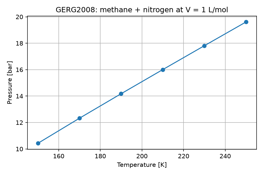
This figure is a scan of the model at one volume. It is an illustration of the API, not a validation dataset: compare the curve with experimental data for the mixture before drawing conclusions from it.
Implementation details
Gerg2008 extends ArModelAdiff, so all the standard ArModel methods are
available, including pressure, volume, lnphi_pt, the residual property
routines and the phase-equilibrium routines.
The model is evaluated with automatic differentiation using hyperdual numbers, so first and second derivatives with respect to amount, volume and temperature come from the same code path.
The volume method is specialized: it uses a Newton solver in log-volume,
initialized with the Soave-Redlich-Kwong volume. This is necessary because the
GERG2008 Helmholtz function does not provide a simple analytical covolume. The
root selection "liquid", "vapor" and "stable" behaves as in the other
models: "stable" compares the Gibbs energy of the two roots.
The model overrides ln_activity_coefficient: each pure-fluid reference is
evaluated with a separate one-component GERG2008 model.
Interpretation, checks and pitfalls
Useful checks on a first run:
- Ideal-gas limit. Increase the volume at fixed temperature and
composition; the pressure must approach
sum(n)*R*T/Vand . - Order independence of the result. Building the model with the components in the opposite order and swapping the amounts accordingly gives the same pressure to machine precision. A different answer means the composition vector no longer matches the model order.
- Component sanity.
model%components%tcand%pccome from the tables, not from your input, and are a quick way to confirm that the right components were selected. - Root verification. After
volume, callpressurewith the returned volume and compare with the requested pressure.
Pitfalls specific to this model:
- A failed volume solve returns a negative volume. The solver returns instead of a physical volume when Newton iteration does not converge. Always check that the volume is positive before using it; a negative volume propagated into a pressure call gives a meaningless number rather than an error.
- No user parameters. There is no way to supply your own pure-component
coefficients or binary interactions to
gerg_2008. If you need them, use a model that accepts them, such as a cubic EOS with mixing rules or PC-SAFT. - Departure functions are limited. As listed above, many pairs have no departure function. Mixtures such as methane + water or carbon dioxide + water are therefore described only through the reducing functions.
- The model is a fixed parameterization. It was developed for natural-gas mixtures. Using it far outside that range is possible but the original parameterization no longer guarantees accuracy.
- A converged calculation is not a validated one. Solver convergence says nothing about whether the model describes your system; that requires comparison with experimental data.
Limits of the model versus limits of the solver
These are different failures and deserve different responses:
| Symptom | Likely cause | What to do |
|---|---|---|
| Volume solve returns | Newton iteration did not converge | Check that the state is inside the model’s range; try a different root_type |
| Bubble or flash routine fails to converge | Phase-equilibrium solver, not the model | Supply better initial guesses (p0, y0, t0) or a better starting state |
| Converged but implausible result | Model or parameters unsuitable for the system | Compare with data; check the component set and the pair coverage listed above |
Next reading
- Thermodynamic fundamentals for amounts, compositions, units and the difference between a model and a solver.
- Saturation points for bubble and dew points and the checks that apply to them.
- GERG2008 parameters for the complete tables of pure-fluid constants and coefficients, binary reducing parameters and departure functions.
- Cubic EOS when you need to supply your own critical data and binary interactions, or when cost matters.
References
- Kunz, O., & Wagner, W. (2012). The GERG-2008 wide-range equation of state for natural gases and other mixtures: an expansion of GERG-2004. Journal of Chemical & Engineering Data, 57(11), 3032-3091.
app/gerg_properties.f90contains a runnable property calculation.