Fitting interaction parameters of binary systems
Sometimes Equations of State needs an extra help to better predict behaviours.
Let’s see how we can optimize binary interaction parameters of a Cubic Equation, using equilibria data.
Data structure
For all the default approachs of parameter optimization the datapoints must be in the format of a pandas DataFrame, with the following columns:
kind: Which kind of point is defined["bubble", "dew", "liquid-liquid", "PT"].T: Temperature (in Kelvin).P: Pressure (in bar).x1: Mole fraction of component 1 (lightest component) in heavy phase.y1: Mole fraction of component 1 (lightest component) in light phase.
In the following cell we import the datapoints from a .csv file
[1]:
import pandas as pd

df = pd.read_csv('./data/CO2_C6.csv')
df
[1]:
| kind | T | P | x1 | y1 | |
|---|---|---|---|---|---|
| 0 | bubble | 303.15 | 20.24 | 0.2385 | 0.9721 |
| 1 | bubble | 303.15 | 30.36 | 0.3698 | 0.9768 |
| 2 | bubble | 303.15 | 39.55 | 0.5063 | 0.9815 |
| 3 | bubble | 303.15 | 50.95 | 0.7078 | 0.9842 |
| 4 | bubble | 303.15 | 57.83 | 0.8430 | 0.9855 |
| 5 | bubble | 303.15 | 64.68 | 0.9410 | 0.9884 |
| 6 | bubble | 303.15 | 67.46 | 0.9656 | 0.9909 |
| 7 | bubble | 315.15 | 20.84 | 0.2168 | 0.9560 |
| 8 | bubble | 315.15 | 30.40 | 0.3322 | 0.9660 |
| 9 | bubble | 315.15 | 40.52 | 0.4446 | 0.9748 |
| 10 | bubble | 315.15 | 50.66 | 0.5809 | 0.9753 |
| 11 | bubble | 315.15 | 60.29 | 0.7180 | 0.9753 |
| 12 | bubble | 315.15 | 69.11 | 0.8457 | 0.9764 |
| 13 | bubble | 315.15 | 72.89 | 0.8928 | 0.9773 |
| 14 | bubble | 315.15 | 75.94 | 0.9252 | 0.9777 |
| 15 | bubble | 315.15 | 77.50 | 0.9424 | 0.9768 |
| 16 | bubble | 315.15 | 78.66 | 0.9520 | 0.9756 |
Default model prediction
Before starting to fit BIPs, let’s see how the model predicts without BIPs.
First, let’s define the model
[2]:
import yaeos

Tc = [304.1, 504.0]
Pc = [73.75, 30.12]
w = [0.4, 0.299]

model = yaeos.PengRobinson76(Tc, Pc, w)
Claculation of Pxy diagrams
Now that the model is defined, lets calculate Pxy diagrams for each temperature.
First, we find the unique values of temperature to iterate over them later.
[3]:
Ts = df["T"].unique()
Ts
[3]:
array([303.15, 315.15])
[4]:
import matplotlib.pyplot as plt
z0 = [0, 1]
zi = [1, 0]
pxs = []
gpec = yaeos.GPEC(model)
for T in Ts:
msk = df["T"] == T
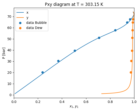
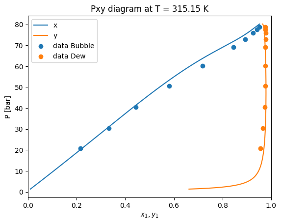
pxy = gpec.plot_pxy(T)
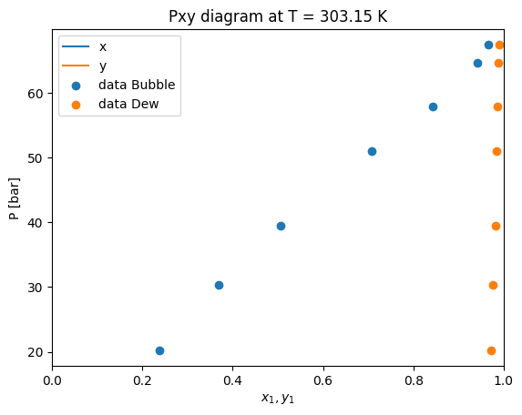
plt.scatter(df[msk]["x1"], df[msk]["P"], label="Bubble Points")
plt.scatter(df[msk]["y1"], df[msk]["P"], label="Dew Points")
plt.xlim(0, 1)
plt.legend()
plt.show()
Here we can see that the PengRobinson EoS present a negative deviation with respect to the experimental points. Let’s se how we can improve these predictions.
Definition of the optimization problem
Now that we already have our data points defined. We need to define the optimization problem.
The yaeos.fitting package includes the BinaryFitter object, this object encapsulates all the logic that is needed to fit binary systems.
[5]:
import yaeos
from yaeos.fitting import BinaryFitter

?BinaryFitter
Model setter function
Looking at the object’s documentation we can see that we need to define a function model_setter that takes the vector of fitting parameters and extra required arguments.
[6]:
def fit_kij(x, model):
    """Fit kij function.

    Args:
        x (list): kij value.
        model (yaeos.CubicEoS): CEOS model that will be fitted
    """
    kij = x[0]

    kij_matrix = [
        [0, kij],
        [kij, 0]
    ]

    lij = [
        [0, 0],
        [0, 0]
    ]

    mixrule = yaeos.QMR(kij=kij_matrix, lij=lij)

    model.set_mixrule(mixrule)

    return model
[7]:
problem = BinaryFitter(
    model_setter=fit_kij,
    model_setter_args=(model,),
    data=df,
    verbose=True
)

x0 = [0.0]

problem.fit(x0, bounds=None)
1 1.7427277515958346 [0.]
2 1.7367297572626244 [0.00025]
3 1.7307370080649485 [0.0005]
4 1.72474952538773 [0.00075]
5 1.712790445469462 [0.00125]
6 1.700852689778661 [0.00175]
7 1.6770418462495278 [0.00275]
8 1.6533183947480148 [0.00375]
9 1.6061393533646415 [0.00575]
10 1.559327111499111 [0.00775]
11 1.4668506368944916 [0.01175]
12 1.3759871697248645 [0.01575]
13 1.1995171255846175 [0.02375]
14 1.030807090584202 [0.03175]
15 0.7207125515768745 [0.04775]
16 0.45494890342547334 [0.06375]
17 0.1633296153190301 [0.09575]
18 0.22052696455206036 [0.12775]
19 0.22052696455206036 [0.12775]
20 0.09792206166179376 [0.11175]
21 0.22052696455206036 [0.12775]
22 0.11825669217983152 [0.10375]
23 0.10598288555962829 [0.11975]
24 0.09823429765712599 [0.11575]
25 0.10459879842351241 [0.10775]
26 0.09712360613884066 [0.11375]
27 0.09823429765712599 [0.11575]
28 0.09730049165208345 [0.11275]
29 0.05599850855641941 [0.11475]
30 0.09823429765712599 [0.11575]
31 0.09823429765712599 [0.11575]
32 0.05537507866049399 [0.11425]
33 0.09712360613884066 [0.11375]
34 0.05567258588798029 [0.1145]
35 0.05510588012730981 [0.114]
36 0.09712360613884066 [0.11375]
37 0.09712360613884066 [0.11375]
38 0.05523694758807889 [0.114125]
39 0.054981862883314914 [0.113875]
40 0.09712360613884066 [0.11375]
41 0.09712360613884066 [0.11375]
42 0.05504299106424188 [0.1139375]
Optimization result
Now that we have fitted the parameter, let’s see the solution. For this, we can see the solution property of the problem. Where we can see that the optimization terminated succesfully with a kij value of around 0.113
[8]:
problem.solution
[8]:
       message: Optimization terminated successfully.
       success: True
        status: 0
           fun: 0.054981862883314914
             x: [ 1.139e-01]
           nit: 21
          nfev: 42
 final_simplex: (array([[ 1.139e-01],
                       [ 1.139e-01]]), array([ 5.498e-02,  5.504e-02]))
Obtain the fitted model
Now that the problem has been optimized, let’s redefine our model with the solution. For this, we use the _get_model method inside of the BinaryFitter object. This just uses the function that we have provided originally (fit_kij)
[9]:
model = problem._get_model(problem.solution.x, model)
Make predictions
Let’s repeat the calculation of Pxy diagrams that we have done earlier
[10]:
import matplotlib.pyplot as plt
z0 = [0, 1]
zi = [1, 0]
pxs = []
gpec = yaeos.GPEC(model)
for T in Ts:
msk = df["T"] == T
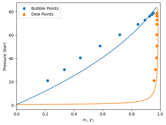
pxy = gpec.plot_pxy(T)
plt.scatter(df[msk]["x1"], df[msk]["P"], label="Bubble Points")
plt.scatter(df[msk]["y1"], df[msk]["P"], label="Dew Points")
plt.xlim(0, 1)
plt.legend()
plt.show()