Gerg2008

In yaeos the multifluid equation \(GERG2008\) residual term is implemented.

import yaeos
import numpy as np
import matplotlib.pyplot as plt

The GERG2008 object is instantiated by providing a list of the components desired to include. The available components are:

• methane

• nitrogen

• carbon dioxide

• ethane

• propane

• n-butane

• isobutane

• n-pentane

• isopentane

• n-hexane

• n-heptane

• n-octane

• nonane

• decane

• hydrogen

• oxygen

• carbon monoxide

• water

• hydrogen sulfide

• helium

• argon

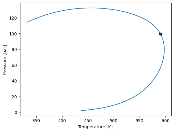
For example, we will calculate the phase envelope for the ternary system of methane, n-butane and decane.

# Define the model to use
model = yaeos.GERG2008(["methane", "n-butane", "decane"])

# Calculate the phase envelope at a specific composition
z = [0.4, 0.2, 0.4]
env = model.phase_envelope_pt(z, kind="dew", max_points=800, t0=400, p0=2)
env.plot()

Things to be careful about

Multiple volume roots

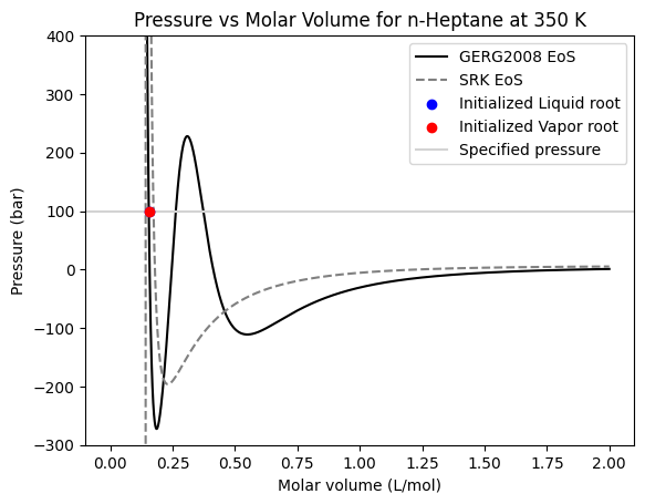
Due to it’s multiparametric nature, the GERG2008 can also be the source of unexpected and undesired errors in modelling. One of the most common cases is the precense of multiple unrealistic volume roots. In this example we show how the isotherm of pure n-Heptane can present an unrealistic root.

When we draw the isotherm at \(350~K\) we can see that there are three possible volume roots for pressures from \(0 bar\) to near \(250 bar\). The middle root does not satisfy the mechanically stability criteria (\(dP/dV\) should be negative) but the other two roots do. But, if we pay attention to the root at higher molar volumes, we can see that it is an unrealistic vapor root that’s just an artifact of the complexity of the GERG2008 equation, and it should not be taken into account.

In yaeos, we use the \(SRK\) equation of state to initialize liquid and vapor volumes, so in most cases we should not end on those unrealisic roots. This is shown in this example, where both the (initialized as) liquid and vapor roots end up in the realistic liquid root. But extra care should be taken when calculating these kind of roots, because this method is not perfect.

import matplotlib.pyplot as plt
import numpy as np
import yaeos

model = yaeos.GERG2008(["n-heptane"])

Tc =  [540.2]
Pc =  [27.4]
w =  [0.349469]

srk = yaeos.SoaveRedlichKwong(Tc, Pc, w)

T = 350  # Temperature in Kelvin
P = 100  # Pressure in bar

# Define a range of molar volumes to calculate pressures
vs = np.linspace(1e-3, 2, 10000)

# Calculate pressures for the specified molar volumes using the GERG2008 model
ps = [model.pressure([1], v, T) for v in vs]

# Calculate pressures using the SRK EoS for comparison
ps_srk = [srk.pressure([1], v, T) for v in vs]

# Calculate the liquid and vapor roots at the specified pressure and temperature
v_liq = model.volume([1], P, T, root="liquid")
v_vap = model.volume([1], P, T, root="vapor")

# Plotting the results
plt.ylim(-300, 400)
plt.plot(vs, ps, color="black", label="GERG2008 EoS")
plt.plot(vs, ps_srk, linestyle="--", color="gray", label="SRK EoS")

plt.scatter(v_liq, P, color="blue", label="Initialized Liquid root", zorder=10)
plt.scatter(v_vap, P, color="red", label="Initialized Vapor root", zorder=10)

plt.axhline(P, color="lightgray", linestyle="-", label="Specified pressure")
plt.xlabel("Molar volume (L/mol)")
plt.ylabel("Pressure (bar)")
plt.title("Pressure vs Molar Volume for n-Heptane at {T} K".format(T=T))
plt.legend()
plt.show()